
Air pollutants rarely stay where they are emitted. Once released from a smokestack, tailpipe, wildfire, field, ship, or solvent, they are carried, diluted, transformed, deposited, and sometimes concentrated again by the atmosphere. Understanding how air pollutants travel through the atmosphere is central to atmospheric science because transport determines who is exposed, where ecosystems are damaged, how cities plan controls, and why pollution can cross borders and oceans. This hub article explains the core processes that move pollutants through air, the chemical changes that occur along the way, the measurement tools scientists use, and the major atmospheric science topics that connect to transport, weather, climate, and human health.
In practical terms, air pollutants include gases such as nitrogen oxides, sulfur dioxide, ozone, carbon monoxide, volatile organic compounds, and ammonia, as well as particles known as particulate matter or aerosols. Travel through the atmosphere refers to the full pathway from emission to final fate: near-source dispersion, vertical mixing, long-range transport, chemical transformation, and removal by dry or wet deposition. I have worked with air quality datasets where a monitor spike initially looked local, then trajectory analysis showed the plume had traveled hundreds of kilometers overnight. That pattern is common. Pollution episodes are often the product of both local emissions and atmospheric transport.
This matters because distance changes risk. Fine particles smaller than 2.5 micrometers can remain suspended for days to weeks, allowing regional transport, while coarse dust may settle more quickly near its source. Ozone is often not emitted directly at ground level but formed downwind through sunlight-driven reactions involving nitrogen oxides and volatile organic compounds. Mercury can circulate globally. Smoke from Canadian wildfires can degrade air quality in the eastern United States. Saharan dust can reach the Caribbean and the Americas. Farmers, city planners, regulators, and public health agencies all rely on atmospheric science to predict these movements and reduce harm.
For readers building a broader understanding of environmental science, atmospheric science is the hub that connects emissions, weather, chemistry, exposure, regulation, and climate. It includes boundary layer meteorology, cloud processes, radiative balance, aerosol physics, dispersion modeling, satellite remote sensing, and source attribution. If you want to understand why one neighborhood experiences higher nitrogen dioxide near highways, why mountain valleys trap winter smoke, or why regional haze persists even after local controls improve, the answer lies in how pollutants move through the atmosphere. The sections below provide the framework used by scientists and air quality professionals.
Emission Sources and the First Stage of Transport
Every transport story begins with a source. Point sources include power plants, refineries, cement kilns, and industrial stacks. Line sources include highways, rail corridors, and shipping lanes. Area sources include agricultural fields, construction sites, urban solvent use, and residential wood burning. Natural sources matter too: volcanoes emit sulfur gases and ash, wetlands emit methane, deserts generate mineral dust, forests release biogenic volatile organic compounds, and wildfires inject enormous amounts of smoke. Source characteristics strongly affect travel. Emission height, exit velocity, temperature, particle size, and release timing all determine whether a pollutant stays near the ground or rises into faster-moving air aloft.
Hot exhaust from a tall stack often forms a plume that rises above the release point because of buoyancy and momentum. This plume rise can reduce immediate ground-level concentrations close to the source, but it may increase impacts farther downwind once the plume mixes downward. Traffic emissions are different. They begin near breathing level and interact with buildings, street canyons, and stop-and-go flow, creating intense local gradients in nitrogen dioxide, ultrafine particles, and black carbon. In field studies near major roads, concentrations can drop sharply within a few hundred meters, showing how the first stage of transport is controlled by micro-scale turbulence and obstacle-driven mixing.
Pollutants are also classified by whether they are primary or secondary. Primary pollutants are emitted directly, such as sulfur dioxide, elemental carbon, or dust. Secondary pollutants form in air, such as ozone, sulfate, nitrate, and secondary organic aerosol. This distinction matters because a source can affect air quality far away without directly emitting the pollutant measured there. For example, power plant sulfur dioxide can oxidize into sulfate particles downwind, and vehicle and solvent emissions can create ozone many kilometers from an urban core. Atmospheric science therefore evaluates both emitted mass and what that mass becomes during transport.
Wind, Turbulence, and the Boundary Layer
The main conveyor belt for air pollutants is wind, but wind alone does not explain concentration patterns. Turbulence, atmospheric stability, and boundary layer depth control how rapidly emissions dilute. The planetary boundary layer is the lowest part of the atmosphere directly influenced by the surface, usually responding to heating, cooling, roughness, and moisture over timescales of about an hour or less. During sunny afternoons, surface heating creates convective turbulence that mixes pollutants upward through a deeper layer, often lowering near-surface concentrations. At night, cooling produces a shallower, more stable layer, which can trap emissions near the ground and raise concentrations by morning.
Atmospheric stability is commonly described by whether air parcels resist or encourage vertical motion. Stable air suppresses mixing, neutral air allows moderate dispersion, and unstable air promotes vigorous mixing. One reason winter pollution episodes can become severe is that cold, stable air and weak winds limit dilution. Temperature inversions are especially important. Under an inversion, air temperature increases with height over a shallow layer instead of decreasing, acting like a lid. Valleys such as Salt Lake City or parts of northern India can experience persistent inversions that trap particulate pollution for days. Once the inversion breaks, concentrations can fall quickly.
Local terrain and land use complicate transport further. Sea breezes move inland during the day and can recirculate pollutants back toward coastal cities. Mountain-valley circulations carry air upslope in daytime and downslope at night. Urban heat islands alter mixing and convergence. Buildings create wakes and vortices that change dispersion around street level. In practice, forecasters often combine surface meteorology, upper-air soundings, and high-resolution models to understand these effects. A monitor reading means little without context about the mixing depth and the structure of the lower atmosphere at the time of measurement.
Chemical Transformation During Transport
Air pollution transport is never just movement; it is movement plus chemistry. Sunlight, oxidants, humidity, and temperature continuously transform pollutants. The hydroxyl radical is often called the atmosphere’s detergent because it initiates oxidation of many gases. Nitrogen oxides and volatile organic compounds react in the presence of sunlight to form ground-level ozone. Sulfur dioxide can oxidize to sulfuric acid and then sulfate aerosol. Ammonia reacts with nitric and sulfuric acids to form ammonium nitrate and ammonium sulfate particles. Organic vapors from vehicles, industry, vegetation, and fires can become secondary organic aerosol through multi-step oxidation.
These reactions alter both toxicity and travel distance. Ozone can peak downwind of the urban emissions that created it, which is why suburban and rural areas often record high summer ozone despite lower local traffic. Fine secondary particles can persist longer and travel farther than some of their precursor gases. Smoke also ages chemically. Fresh wildfire smoke may be rich in organic carbon and specific tracers, while older smoke can become more oxidized and produce elevated ozone. In several North American fire seasons, cities far from the flames experienced harmful PM2.5 because atmospheric transport and chemistry converted a distant fire into a regional air quality emergency.
Humidity and clouds also matter. Aqueous-phase chemistry inside cloud droplets can accelerate sulfate formation, and fog can concentrate certain pollutants near the surface. Sun angle and seasonal daylight affect photochemistry, which helps explain why ozone is usually a warm-season problem while nitrate particles often rise in cooler months. Scientists represent these processes with chemical transport models such as CMAQ, CAMx, GEOS-Chem, and WRF-Chem. These tools solve emissions, meteorology, transport, and chemistry together, allowing researchers to estimate how much of a measured pollutant came from local sources, distant sources, or atmospheric formation during transit.
Deposition, Lifetime, and Long-Range Transport
How far a pollutant travels depends largely on its atmospheric lifetime. Lifetime is the average time a substance remains in air before being removed by chemistry or deposition. Carbon monoxide can remain for weeks to months, enabling continental transport. Fine aerosol may persist for days to more than a week. Larger particles deposit faster due to gravity. Removal occurs by dry deposition, where gases or particles stick to vegetation, water, soil, or built surfaces, and by wet deposition, where rain or snow scavenges pollutants from the air. Wet deposition is one reason precipitation can sharply improve visibility after a haze event.
The combination of lifetime and wind patterns explains long-range transport. Sulfate and nitrate haze can move across states and national borders. Asian dust can reach western North America. Persistent organic pollutants and mercury can undergo cycles of transport and deposition over very long distances. The table below summarizes how key factors influence travel.
| Factor | Effect on Pollutant Travel | Example |
|---|---|---|
| Particle size | Smaller particles stay suspended longer | PM2.5 from smoke travels regionally |
| Emission height | Higher release can enter faster winds aloft | Power plant plume impacts downwind counties |
| Atmospheric stability | Stable air limits dilution near the surface | Winter inversion traps wood smoke |
| Chemical reactivity | Reactive gases may transform before removal | NOx and VOCs form ozone downwind |
| Precipitation | Rain and snow remove particles and soluble gases | Storm passage lowers haze concentrations |
| Surface type | Forests and rough surfaces enhance deposition | Ozone uptake by vegetation reduces local levels |
Long-range transport has policy consequences. The 1979 Convention on Long-Range Transboundary Air Pollution in Europe recognized that sulfur and nitrogen emissions could damage lakes and forests far from the source. In the United States, interstate ozone and fine particle transport has shaped federal rules under the Clean Air Act. On a global scale, wildfire smoke, dust, and industrial emissions are now tracked continuously by satellites such as MODIS, VIIRS, TROPOMI, and GOES. These instruments reveal plumes crossing oceans, but interpreting satellite images still requires ground monitors, meteorological analysis, and transport models to determine what is aloft and what reaches people at the surface.
Measurement, Modeling, and Source Attribution
Scientists answer the question of where pollution came from by combining observations with models. Surface monitoring networks measure criteria pollutants, PM2.5 mass, ozone, nitrogen dioxide, sulfur dioxide, carbon monoxide, and meteorological variables. Speciation networks add sulfate, nitrate, ammonium, organic carbon, elemental carbon, metals, and molecular tracers. Lidar can profile aerosol layers vertically. Radiosondes measure temperature and wind aloft. Satellite retrievals estimate aerosol optical depth, nitrogen dioxide columns, and smoke extent. Each method has strengths and limits. A ground monitor gives accurate local concentration, while a satellite provides broad coverage but not a direct surface reading.
Source attribution typically uses several techniques together. Back-trajectory models such as HYSPLIT estimate where an air parcel traveled before reaching a site. Receptor models like Positive Matrix Factorization identify source fingerprints within measured particle chemistry. Eulerian chemical transport models simulate emissions and atmospheric processes over a grid. Isotopic analysis can separate some natural and anthropogenic sources. In applied work, I treat no single method as decisive. If trajectories, satellite imagery, fire detections, and speciated PM all point to aged wildfire smoke, confidence is high. If only one indicator points that way, the conclusion should stay provisional.
This analytical framework supports forecasting and regulation. Air agencies issue smoke outlooks, ozone alerts, and particulate advisories based on expected transport and chemistry. Industries use dispersion models such as AERMOD for permitting and compliance near sources. Emergency managers use plume models during chemical releases. Researchers evaluate control strategies by testing scenarios: What happens to ozone if nitrogen oxides fall but volatile organic compounds do not? How much PM2.5 declines if ammonia emissions from agriculture are reduced? Because the atmosphere is nonlinear, the answer depends on place, season, and the chemical regime, which is why careful attribution matters.
Why Atmospheric Transport Connects the Whole Environmental Science Topic
Atmospheric science sits at the center of environmental science because air transport links systems that are often studied separately. Human health depends on exposure, not just emissions. Ecology depends on where nitrogen and sulfur are deposited. Water quality can be affected by atmospheric mercury and nutrient deposition. Climate interacts with pollutants because aerosols scatter and absorb radiation, black carbon darkens snow, and heat alters ozone formation and wildfire behavior. Land management influences dust and smoke. Energy policy changes emissions profiles. Transportation planning shapes near-road exposure. Few environmental problems remain local once the atmosphere becomes the pathway.
For readers using this page as a hub, the major atmospheric science branches to explore next are meteorology, atmospheric chemistry, aerosol science, air quality monitoring, dispersion modeling, remote sensing, climate interactions, and environmental health. Learn the scales first: local, urban, regional, continental, and global. Then learn the governing processes: emission, advection, diffusion, convection, chemical transformation, and deposition. Finally, learn the evidence chain: measurements, trajectories, models, and source fingerprints. With that structure, individual topics such as acid rain, urban smog, wildfire smoke, dust storms, or indoor-outdoor exchange become much easier to understand.
The most important takeaway is simple: air pollution is dynamic. What people breathe today may have been emitted yesterday in another city, another state, or another country, then altered by sunlight, humidity, and clouds before reaching ground level. Better decisions come from recognizing that movement. If you are building your understanding of environmental science, use atmospheric science as the organizing framework, then follow the linked subtopics on chemistry, monitoring, weather, health, and policy to deepen your knowledge.
Frequently Asked Questions
What determines how far air pollutants can travel after they are released?
The distance an air pollutant travels depends on a combination of meteorology, chemistry, particle size, and the height at which it enters the atmosphere. Wind speed and wind direction are the most obvious drivers, because they physically move pollution away from its source. However, transport is not just a matter of wind pushing a plume downwind. Atmospheric stability, turbulence, and mixing height all shape how quickly pollutants spread vertically and horizontally. On a well-mixed day, pollution may dilute faster near the surface but also become distributed across a larger air mass. Under stable conditions, especially during temperature inversions, pollutants can remain trapped close to the ground and build up to unhealthy levels.
The lifetime of the pollutant matters just as much as the weather. Short-lived compounds may react, settle, or be washed out before they travel far, while longer-lived gases can cross regions, continents, or even oceans. Fine particles and gases often travel farther than large particles, because heavier particles settle out more quickly due to gravity. Emission height also plays a major role. Pollution released from tall smokestacks or injected high into the atmosphere by wildfires can enter faster-moving air aloft, allowing it to bypass local dilution patterns and travel long distances. In practice, how far pollution goes is the result of multiple processes happening at once: advection by wind, turbulent dispersion, chemical transformation, dry deposition, and wet deposition.
How do weather patterns and atmospheric conditions affect the movement of pollution?
Weather controls pollution transport at nearly every stage. Winds carry pollutants horizontally, while turbulence and convection mix them vertically. During sunny daytime conditions, the ground warms the air above it, creating rising motions that help disperse pollutants through a deeper boundary layer. This often reduces concentrations near the surface, although it can also spread pollution over a wider area. At night, the atmosphere often becomes more stable, especially under clear skies and light winds, which suppresses vertical mixing and allows emissions from traffic, industry, or residential burning to accumulate closer to the ground.
Larger-scale weather systems also matter. High-pressure systems are commonly associated with stagnant air, light winds, and limited dispersion, which can lead to multi-day pollution episodes in urban and industrial areas. Low-pressure systems and fronts can shift wind directions, transport pollutants between regions, and sometimes ventilate polluted air masses. Rain and snow remove many pollutants through wet deposition, while dry conditions allow them to remain airborne longer. Temperature inversions are especially important because they place a layer of warmer air above cooler surface air, acting like a lid that traps pollutants beneath it. In coastal areas, sea breezes can recirculate pollution inland and offshore over the course of a day. In mountainous terrain, valley flows and slope winds can channel pollutants in predictable but complex ways. Altogether, atmospheric conditions determine whether pollution disperses, concentrates, or travels far beyond where it was emitted.
Can air pollutants change chemically while they are traveling through the atmosphere?
Yes, and this is one of the most important concepts in atmospheric science. Many pollutants do not remain in the same form after emission. Instead, they undergo chemical reactions driven by sunlight, oxidants such as hydroxyl radicals, ozone, and nitrate radicals, and interactions with water vapor or cloud droplets. These transformations can create entirely new pollutants that may be more harmful, more persistent, or more easily transported than the original emissions. For example, nitrogen oxides and volatile organic compounds can react in the presence of sunlight to form ground-level ozone, a secondary pollutant that is not emitted directly but is produced in the atmosphere downwind of sources.
Particles also change during transport. Sulfur dioxide can oxidize into sulfate particles, nitrogen oxides can form nitrate particles, and gases from vehicles, industry, vegetation, or wildfires can produce secondary organic aerosols. These reactions affect not only air quality but also visibility, cloud formation, and climate. Chemical aging can change particle size, acidity, and water uptake, which in turn influences how long the particles stay airborne and where they deposit. This is why pollution measured far from a source may look chemically different from what originally came out of a smokestack or tailpipe. It also explains why controlling one pollutant can influence several others, because atmospheric chemistry connects emissions, transport, and exposure in complex ways.
Why does pollution sometimes affect places that are far away from the original source?
Pollution can affect distant locations because the atmosphere is a connected transport system rather than a set of isolated local air sheds. If a pollutant remains airborne long enough, prevailing winds, storm tracks, and large-scale circulation patterns can move it hundreds or thousands of miles. Fine particulate matter, ozone precursors, smoke from major wildfires, dust, and certain industrial emissions are especially known for long-range transport. In some cases, air masses carry pollution across state lines, national borders, and oceans, making air quality a regional or even global issue rather than only a local one.
Distance impacts are also possible because pollutants can be transformed into secondary forms while traveling. A city may emit gases that later become ozone or fine particles in rural areas downwind. Wildfire smoke may start as a dense local plume but then spread over vast regions after lofting into higher layers of the atmosphere. Similarly, emissions from ships can influence coastal air quality, and agricultural emissions can contribute to particle formation far from the fields where they originated. These long-range effects are a major reason why air quality management often requires interstate, international, and sector-wide cooperation. Communities far from major sources may still experience degraded air quality because what matters is not only where pollution is emitted, but also how the atmosphere transports and transforms it over time.
How do scientists track and predict where air pollutants will go?
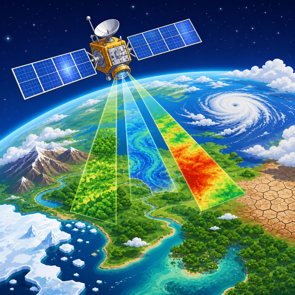
Scientists use a combination of direct measurements, remote sensing, and computer modeling to follow pollutants through the atmosphere. Ground-based monitoring stations measure pollutants such as ozone, particulate matter, nitrogen dioxide, sulfur dioxide, and carbon monoxide at fixed locations. Aircraft, weather balloons, ships, and mobile laboratories provide additional observations aloft and across different environments. Satellites add a broader view by detecting smoke plumes, aerosol loading, trace gases, fire activity, and dust transport over large areas that would be difficult to monitor from the ground alone. Together, these observations help researchers identify source regions, follow transport pathways, and assess where populations and ecosystems may be exposed.
To predict movement, scientists use atmospheric transport and chemistry models that incorporate emissions data, weather forecasts, topography, and chemical reaction mechanisms. These models simulate advection by winds, turbulent mixing, deposition to land and water, and chemical transformation during transport. Some are designed for local plume studies near roads, factories, or ports, while others operate at regional to global scales to evaluate smoke events, transboundary pollution, or seasonal ozone formation. Forecast systems are especially useful for public health alerts and regulatory planning because they can estimate when and where concentrations may rise. Although there is always uncertainty due to changing weather, incomplete emissions inventories, and complex chemistry, modern monitoring networks and models provide a powerful, evidence-based picture of how pollutants move through the atmosphere and why their impacts are often felt far from where they began.